Lorentzian with lmfit
Introduction
The objective of this notebook is to show how to use one of the models of the QENSlibrary, lorentzian, to perform some fits.
scipy.optimize.curve_fit is used for fitting.
Physical units
For information about unit conversion, please refer to the jupyter notebook called Convert_units.ipynb in the tools folder.
The dictionary of units defined in the cell below specify the units of the refined parameters adapted to the convention used in the experimental datafile.
[1]:
# Units of parameters for selected QENS model and experimental data
dict_physical_units = {"omega": "1/ps",
                       'scale': "unit_of_signal.ps",
                       'center': "1/ps",
                       'hwhm': "1/ps"}
Import libraries
[2]:
import numpy as np
import ipywidgets
import matplotlib.pyplot as plt
from scipy.optimize import curve_fit
import ipywidgets
import QENSmodels
Plot fitting model
The widget below shows the lorentzian peak shape function imported from QENSmodels where the function’s parameters Scale, Center and FWHM can be varied.
[3]:
# Dictionary of initial values
ini_parameters = {'scale': 5., 'center': 5., 'hwhm': 3.}

def interactive_fct(scale, center, hwhm):
    """
    Plot to be updated when ipywidgets sliders are modified
    """
    xs = np.linspace(-10, 10, 100)

    fig0, ax0 = plt.subplots()
    ax0.plot(xs, QENSmodels.lorentzian(xs, scale, center, hwhm))
    ax0.set_xlabel('x')
    ax0.grid()

# Define sliders for modifiable parameters and their range of variations
scale_slider = ipywidgets.FloatSlider(value=ini_parameters['scale'],
                                      min=0.1, max=10, step=0.1,
                                      description='scale',
                                      continuous_update=False)

center_slider = ipywidgets.IntSlider(value=ini_parameters['center'],
                                     min=-10, max=10, step=1,
                                     description='center',
                                     continuous_update=False)

hwhm_slider = ipywidgets.FloatSlider(value=ini_parameters['hwhm'],
                                     min=0.1, max=10, step=0.1,
                                     description='hwhm',
                                     continuous_update=False)

grid_sliders = ipywidgets.HBox([ipywidgets.VBox([scale_slider, center_slider]),
                                ipywidgets.VBox([hwhm_slider])])

# Define function to reset all parameters' values to the initial ones
def reset_values(b):
    """
    Reset the interactive plots to inital values.
    """
    scale_slider.value = ini_parameters['scale']
    center_slider.value = ini_parameters['center']
    hwhm_slider.value = ini_parameters['hwhm']

# Define reset button and occurring action when clicking on it
reset_button = ipywidgets.Button(description = "Reset")
reset_button.on_click(reset_values)

# Display the interactive plot
interactive_plot = ipywidgets.interactive_output(
    interactive_fct,
    {'scale': scale_slider,
     'center': center_slider,
     'hwhm': hwhm_slider}
)

display(grid_sliders, interactive_plot, reset_button)
Creating reference data
Input: the reference data for this simple example correspond to a Lorentzian with added noise.
The fit is performed using scipy.optimize.curve_fit. The example is based on implementations from https://docs.scipy.org/doc/scipy/reference/generated/scipy.optimize.curve_fit.html
[4]:
# Creation of reference data
nb_points = 100
xx = np.linspace(-10, 10, nb_points)
added_noise = np.random.normal(0, 1, nb_points)
lorentzian_noisy = QENSmodels.lorentzian(
    xx,
    scale=0.89,
    center=-0.025,
    hwhm=0.45
) * (1. + 0.1 * added_noise) + 0.01 * added_noise

fig1, ax1 = plt.subplots()
ax1.plot(xx, lorentzian_noisy, label='reference data')
ax1.set_xlabel('x')
ax1.grid()
ax1.legend();

Setting and fitting
From https://docs.scipy.org/doc/scipy/reference/generated/scipy.optimize.curve_fit.html
[5]:
initial_parameters_values = [1, 0.2, 0.5]

fig2, ax2 = plt.subplots()
ax2.plot(xx, lorentzian_noisy, 'b-', label='reference data')
ax2.plot(
    xx,
    QENSmodels.lorentzian(xx, *initial_parameters_values),
    'r-',
    label='model with initial guesses'
)
ax2.set_xlabel('x')
ax2.legend(bbox_to_anchor=(0., 1.15), loc='upper left', borderaxespad=0.)
ax2.grid();

[6]:
popt, pcov = curve_fit(QENSmodels.lorentzian, xx, lorentzian_noisy, p0=initial_parameters_values)
Plotting the results
[7]:
# Calculation of the errors on the refined parameters:
perr = np.sqrt(np.diag(pcov))

print(f"Values of refined parameters:\nscale: {popt[0]} +/- {perr[0]} {dict_physical_units['scale']}\n"
      f"center: {popt[1]} +/- {perr[1]} {dict_physical_units['center']}\n"
      f"HWHM: {popt[2]} +/- {perr[2]} {dict_physical_units['hwhm']}")
Values of refined parameters:
scale: 0.8401433663930493 +/- 0.015271146793198383 unit_of_signal.ps
center: -0.018478686118974085 +/- 0.007422705328117259 1/ps
HWHM: 0.4094755075815917 +/- 0.010543965084163493 1/ps
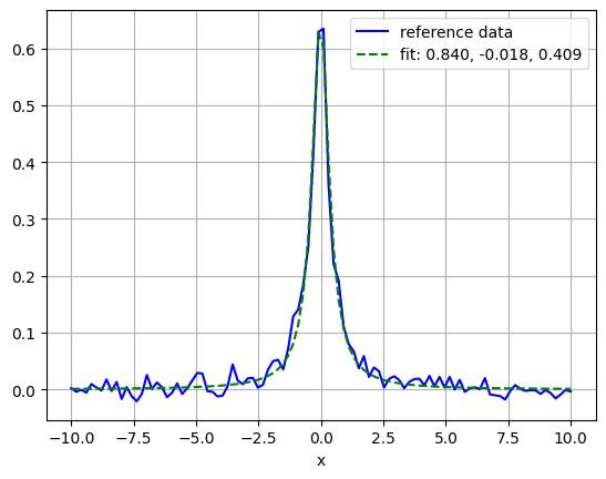
[8]:
 # Comparison of reference data with fitting result
fig3, ax3 = plt.subplots()
ax3.plot(xx, lorentzian_noisy, 'b-', label='reference data')
ax3.plot(
    xx,
    QENSmodels.lorentzian(xx, *popt),
    'g--',
    label='fit: %5.3f, %5.3f, %5.3f' % tuple(popt))
ax3.legend()
ax3.set_xlabel('x')
ax3.grid();
[ ]: