Two Lorentzian ∗ resolution with lmfit

Introduction

The objective of this notebook is to show how to use one of the models of the QENSlibrary, Lorentzian, to perform some fits. lmfit is used for fitting.

The following example uses the data from IRIS: - workspace_index=0, file: irs26176_graphite002_red.nxs

- related instrument resolution data irs26173_graphite002_res.nxs

The ISIS sample datasets can be downloaded from Mantid’s website. The data used for this example are in the sample datafile: data_2lorentzians.dat and the instrument resolution datafile irf_iris.dat, respectively.

This example is based on a Mantid “Fitting QENS Peaks” tutorial.

The implementation with lmfit is based on https://lmfit.github.io/lmfit-py/model.html

This example requires an additional Python module scipy.interpolate to interpolate the tabulated data of the instrument resolution.

Physical units

For information about unit conversion, please refer to the jupyter notebook called Convert_units.ipynb in the tools folder.

The dictionary of units defined in the cell below specify the units of the refined parameters adapted to the convention used in the experimental datafile.

# Units of parameters for selected QENS model and experimental data
dict_physical_units = {'omega': "meV",
                       'q': "1/Angstrom",
                       'hwhm': "meV",
                       'scale': "unit_of_signal.meV",
                       'center': "meV"}

Import libraries

import numpy as np
import matplotlib.pyplot as plt
import ipywidgets
import lmfit
from scipy.interpolate import interp1d
import QENSmodels

path_to_data = './data/'

Step 1: load instrument resolution data

irf_iris = np.loadtxt(path_to_data + 'irf_iris.dat')
x_irf = irf_iris[:, 0]
y_irf = irf_iris[:, 1]

Step 2: create function for instrument resolution data (cubic interpolation between tabulated data points)

Create model: 2 lorentzians convoluted with instrument resolution: 6 parameters

def irf_gate(x):
    """
    Function defined from the interpolation of instrument resolution data
    Used to define fitting model and plot
    """
    f = interp1d(x_irf, y_irf, kind='cubic', bounds_error=False, fill_value='extrapolate')

    return f(x)

# plot tabulated data and interpolated data
xx = np.linspace(-.25, .25, 500)

fig0 = plt.figure()
plt.plot(x_irf, y_irf, 'b.', label='tabulated data')
plt.plot(xx, irf_gate(xx), 'g--', label='extrapolated data')
plt.legend()
plt.xlabel('Energy transfer (meV)')
plt.title('Instrument resolution: plot tabulated data and interpolated data')
plt.grid();

Step 3: create “double lorentzian” profile

def model_2lorentzians(x, scale1, center1, hwhm1, scale2, center2, hwhm2):
    return QENSmodels.lorentzian(
        x,
        scale1,
        center1,
        hwhm1
    ) + QENSmodels.lorentzian(
        x,
        scale2,
        center2,
        hwhm2
    )

Step 4: create convolution function

Code from https://github.com/jmborr/qef

def convolve(model, resolution):
    c = np.convolve(model, resolution, mode='valid')
    if len(model) % len(resolution) == 0:
        c = c[:-1]
    return c

class Convolve(lmfit.CompositeModel):
    def __init__(self, resolution, model, **kws):
        super(Convolve, self).__init__(resolution, model, convolve, **kws)
        self.resolution = resolution
        self.model = model

    def eval(self, params=None, **kwargs):
        res_data = self.resolution.eval(params=params, **kwargs)

        # evaluate model on an extended energy range to avoid boundary effects
        independent_var = self.resolution.independent_vars[0]
        e = kwargs[independent_var]  # energy values
        neg_e = min(e) - np.flip(e[np.where(e > 0)], axis=0)
        pos_e = max(e) - np.flip(e[np.where(e < 0)], axis=0)
        e = np.concatenate((neg_e, e, pos_e))
        kwargs.update({independent_var: e})
        model_data = self.model.eval(params=params, **kwargs)

        # Multiply by the X-spacing to preserve normalization
        de = (e[-1] - e[0])/(len(e) - 1)  # energy spacing
        return de * convolve(model_data, res_data)

Step 5: Load reference data - extract x and y values

two_lorentzians_iris = np.loadtxt(path_to_data + 'data_2lorentzians.dat')
xx = two_lorentzians_iris[:, 0]
yy = two_lorentzians_iris[:, 1]

model = Convolve(lmfit.Model(irf_gate), lmfit.Model(model_2lorentzians))

Step 6: Fit

result = model.fit(yy, x=xx, scale1=1., center1=0., hwhm1=0.25, scale2=5., center2=0., hwhm2=0.02)

# plot initial configuration
fig1 = plt.figure()
plt.plot(xx, yy, '+', label='experimental data')
plt.plot(xx, result.init_fit, 'k--', label='initial model')
plt.legend(loc='upper right')
plt.xlabel('Energy transfer (meV)')
plt.title('Plot before fitting: experimental data and mode with initial guesses')
plt.grid();

Step 7: Plotting results

print('Result of fit:\n', result.fit_report())

Result of fit:
 [[Model]]
    (Model(irf_gate) <function convolve at 0x7fa35a393700> Model(model_2lorentzians))
[[Fit Statistics]]
    # fitting method   = leastsq
    # function evals   = 85
    # data points      = 1905
    # variables        = 6
    chi-square         = 0.39263648
    reduced chi-square = 2.0676e-04
    Akaike info crit   = -16155.9415
    Bayesian info crit = -16122.6280
    R-squared          = 0.99839539
[[Variables]]
    scale1:   1.42322195 +/- 0.01978848 (1.39%) (init = 1)
    center1:  0.01133545 +/- 0.00188391 (16.62%) (init = 0)
    hwhm1:    0.15081965 +/- 0.00439638 (2.91%) (init = 0.25)
    scale2:   4.36339870 +/- 0.01712906 (0.39%) (init = 5)
    center2: -0.00111521 +/- 2.8725e-05 (2.58%) (init = 0)
    hwhm2:    0.01651581 +/- 7.3536e-05 (0.45%) (init = 0.02)
[[Correlations]] (unreported correlations are < 0.100)
    C(scale2, hwhm2)    = +0.9192
    C(hwhm1, scale2)    = +0.8056
    C(hwhm1, hwhm2)     = +0.6732
    C(scale1, hwhm2)    = -0.5394
    C(scale1, scale2)   = -0.5372
    C(center1, scale2)  = +0.2989
    C(center1, hwhm1)   = +0.2891
    C(center1, hwhm2)   = +0.2525
    C(center1, center2) = -0.2405

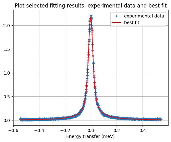
Plot experimental data and best fit using matplotlib.pyplot

fig2 = plt.figure()
plt.plot(xx, yy, '+', label='experimental data')
plt.plot(xx, result.best_fit, 'r-', label='best fit')
plt.grid()
plt.xlabel('Energy transfer (meV)')
plt.title('Plot selected fitting results: experimental data and best fit')
plt.legend();

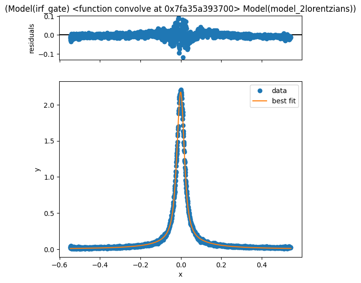
Other option: use lmfit features to plot result

result.plot()

Print values and errors of refined parameters:

for item in result.params.keys():
    print(f'{item[:-1]}: {result.params[item].value} +/- {result.params[item].stderr} {dict_physical_units[item[:-1]]}')

scale: 1.4232219542906104 +/- 0.019788484110928088 unit_of_signal.meV
center: 0.011335450282115963 +/- 0.0018839143254284199 meV
hwhm: 0.15081964541484183 +/- 0.004396377670405706 meV
scale: 4.363398698615817 +/- 0.01712905554857125 unit_of_signal.meV
center: -0.0011152055608803012 +/- 2.8725411337342307e-05 meV
hwhm: 0.016515810379461503 +/- 7.353591551420947e-05 meV

---

Generated by nbsphinx from a Jupyter notebook.